Stitching maps together
In the program SAS.Planet, The image below is pretty much how you want to be selecting certain layers like Z18 Z19 overlapping them. In this example when all 8 captures are stitched together you get a large seamless image of the river corridor down at water level.
I first started off trying to be precise with captures and would of had my borders almost butting each other. This lead to greyed out gaps in my maps with black walls around them. A pixel difference is like a chasm on your plotter. So overlap where you can. In many cases you are guessing where the edge of a prior capture really was as once you move to the next capture. Sure you will see the greyed out boxes of downloaded tiles, but doubt still lingers if you actually overlapped.
I first started off trying to be precise with captures and would of had my borders almost butting each other. This lead to greyed out gaps in my maps with black walls around them. A pixel difference is like a chasm on your plotter. So overlap where you can. In many cases you are guessing where the edge of a prior capture really was as once you move to the next capture. Sure you will see the greyed out boxes of downloaded tiles, but doubt still lingers if you actually overlapped.
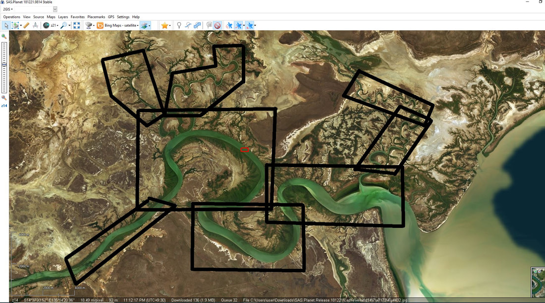 Simulated capture areas overlapping
To actually see this image as a Z18 level in action on your chart plotter, all you would see is the size of the red box on your boats screen.
Let the capturing begin
SAS.Planet
Get your map , check other map types for the best one that suits your requirements. IE some dams have older maps with less water , exposing old logs & rockbars, better resolutions etc.
Select your first capture, download & get ready to stitch the tiles.
The settings are different from the keyhole map process.
The below image I have already gone onto the second capture overlapping and using the polygonal selection tool
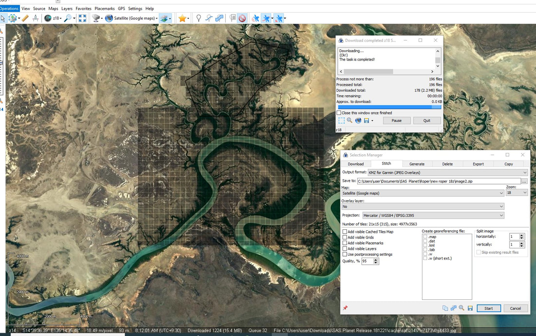
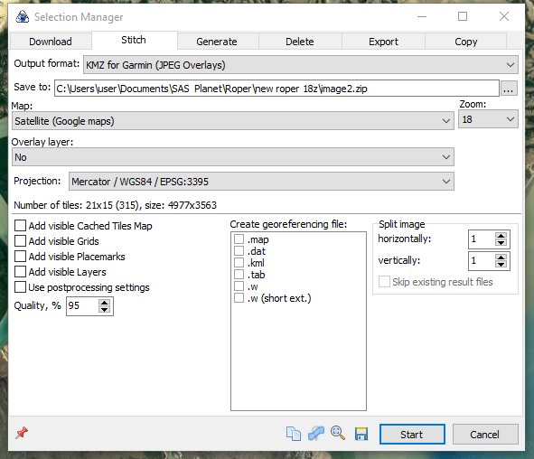
The stitching settings required are Output Format = KMZ for Garmin (JPEG Overlay)
Save to : your folder BUT with a .ZIP extension. (So change the file name from .jpeg to .zip) **
Zoom level in this case is 18
Projector : I use Mercator WGS84 EPSG 3395
You don't need to check the KML checkbox as a .kmz file gets created in the zip file
Save to : your folder BUT with a .ZIP extension. (So change the file name from .jpeg to .zip) **
Zoom level in this case is 18
Projector : I use Mercator WGS84 EPSG 3395
You don't need to check the KML checkbox as a .kmz file gets created in the zip file
Select your sections and repeat the capture & stitch process, remembering to rename each new selection & check your stitch settings in case something changes.
Save your zip files in a folder. In this instance they totalled 8 zip files. The numbering I keep simple with 1,2,3,4,5,6,7,8,9,91,92,93 etc etc. The numbers in sequence are the files for the joining later. If I have been creative & created multiple maps of the same level ie rivermouth1, rivermouth2 & dam1, dam2, dam3 I will split into their sections later. The files should look similar to the below file images (dont worry about file sizes they will be random big & small)
Save your zip files in a folder. In this instance they totalled 8 zip files. The numbering I keep simple with 1,2,3,4,5,6,7,8,9,91,92,93 etc etc. The numbers in sequence are the files for the joining later. If I have been creative & created multiple maps of the same level ie rivermouth1, rivermouth2 & dam1, dam2, dam3 I will split into their sections later. The files should look similar to the below file images (dont worry about file sizes they will be random big & small)
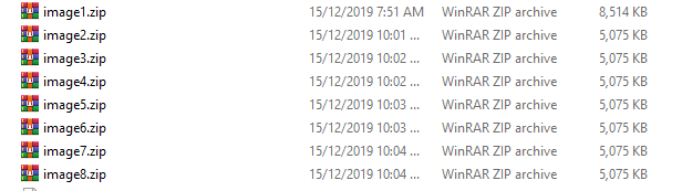
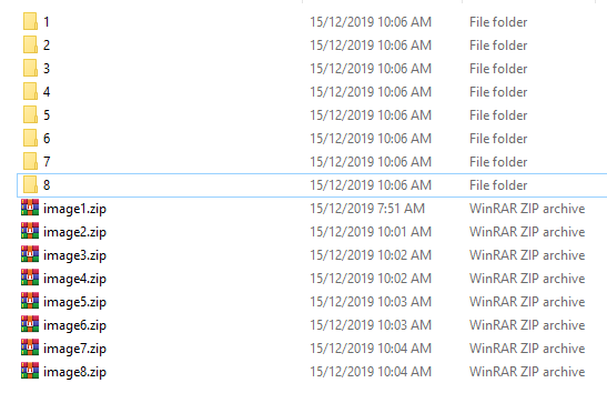
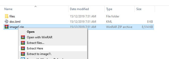
I create corresponding folders to match the zipped files , drag them in to its folder & unzip (extract) in that folder. You end up with a file folder & a .kml (hence the reason not to tick the kml box when stitching) If you don't make new folders for your files everything will get overwritten. It can get a little messy with folders for folders. Make sure you have extracted the zip files in each folder.
Time for Insight Map Creator
Lets get the paperwork done that sets the scene for what we are about to create. Remember in IMC the advanced options tab is how you fine tune your view options.
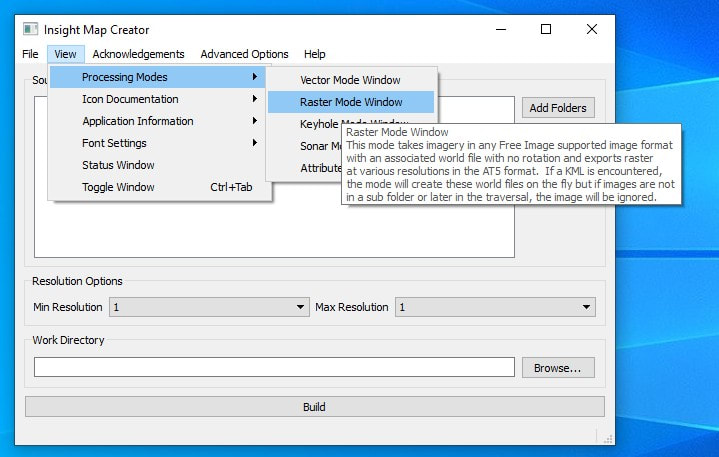
Go to VIEW > Processing Mode > Raster mode Window
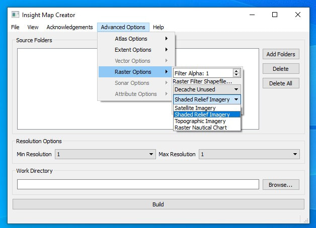
then Advanced Options to fine tune, Advanced Options > Atlas version (I go for 13 for newer model chart plotters) (not sure if it is even required in this processing, but I do it anyway)
Advanced Options > Raster Options > filter alpha 1 (this determines black borders around your images)(so if you see black borders in chart plotter you probably missed this bit)
Raster Options > Shaded Relief Imagery (This is what you have to tell your chart plotter what you have on the card) (and in this case your satellite layers are shaded relief imagery)
Time for Insight Map Creator
Lets get the paperwork done that sets the scene for what we are about to create. Remember in IMC the advanced options tab is how you fine tune your view options.
Go to VIEW > Processing Mode > Raster mode Window
then Advanced Options to fine tune, Advanced Options > Atlas version (I go for 13 for newer model chart plotters) (not sure if it is even required in this processing, but I do it anyway)
Advanced Options > Raster Options > filter alpha 1 (this determines black borders around your images)(so if you see black borders in chart plotter you probably missed this bit)
Raster Options > Shaded Relief Imagery (This is what you have to tell your chart plotter what you have on the card) (and in this case your satellite layers are shaded relief imagery)
OK that's the behind the scenes work done.
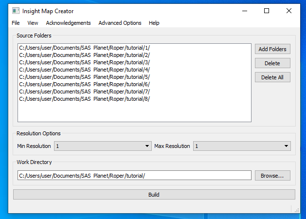
Add your folders. As per image below I added 8 folders that I checked had all been unzipped. There are zip files in these folders that will not be read by IMC. Its only looking for what you unzipped.
Your work folder will need to be named a bit different as it gets confusing where you are at in the process. In your work folder I use folder numbers again for the AT5 files, ie my Z17 sas source folders/files get converted to Z17 AT5 files in IMC and the bounded AT5 outputs are dragged into their Z17 IMC folder so I don't overwrite it (again). (Just be methodical and it will make sense when you get to it)
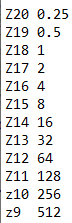
Choose your resolutions. In this case resolution 1 refers to Z18 & I am only going to create one layer for the chart plotter so max & min are the same. ( Chart Above in gallery, I can never find the original chart online)) If I wasn't going to do the whole capture process all over again at Z17 & Z16 Z19 etc I may of used Min & Max resolutions at 1 & 4 or 1 & 8 (meaning IMC would create the other layers from the 8 Z18 folders I supplied.)
Build
After a few minutes depending on processor speed, your Output folder now has a Bound AT5 folder in it. Its contents should look like _3Dtexture_1.at5 (the _1. signifies resolution 1 or Z18 zoom.)
Copy that .at5 file to an sd card , pop into your lowrance chart plotter & go to location and your layer should show up when zoomed in enough.
All done (or is it)
I like my maps zoomable, and so probably do you too.
Start the whole process again in SAS.Planet and pick a few more resolutions, starting with Z12 then Z15 (join a few captures) ( I usually do all my layers in SAS first which may take hours to create file & unpack in respective folders) There is a resolution gap between Z12 & Z15 or what ever zoom you use. Don't worry. Your chart plotter will just stretch the image till it gets to the next zoom layer available. The bigger the gap the more pixilated it will be so you might as well do it right and do each layer.
An example of SAS capture for your zooms in Z12 Might be 6 overlays of the Top End Of Australias Northern Territory & then you might do 18 overlays at Z13 Resolution of the same sort of area (but less wasted sea mass). When processed through to the end with IMC you keep these in a folder called Top End Z12-Z13 and these then become your common files that would add to the SD card if you made maps of other sections of rivers. So how it looks on your chart plotter is ..... a pic of Top End, lets zoom down, down, down.... getting blurryish but still OK.. then "bang" at your main map its crystal clear again as you hit Z16 level you created and zoom down you go.
The thing is, you are not going to really use the Z levels until about 16, unless you are sitting in your boat in the shed & want to check out how your map looks 600 km away as you scroll across to look for your creation or have lots of individual river systems mapped.
